
━━━━━━━━━━━━━━━━━━━━━━━━━━━━━━━━━━━━━━
Assessment 1 – Natural Disaster – Tornado
Useful expressions that I will be using in my project:
- $F – the current frame number
- $T – the current time
example: size x = $T * 2
the size will be the time times two depending on the point in time in your simulation
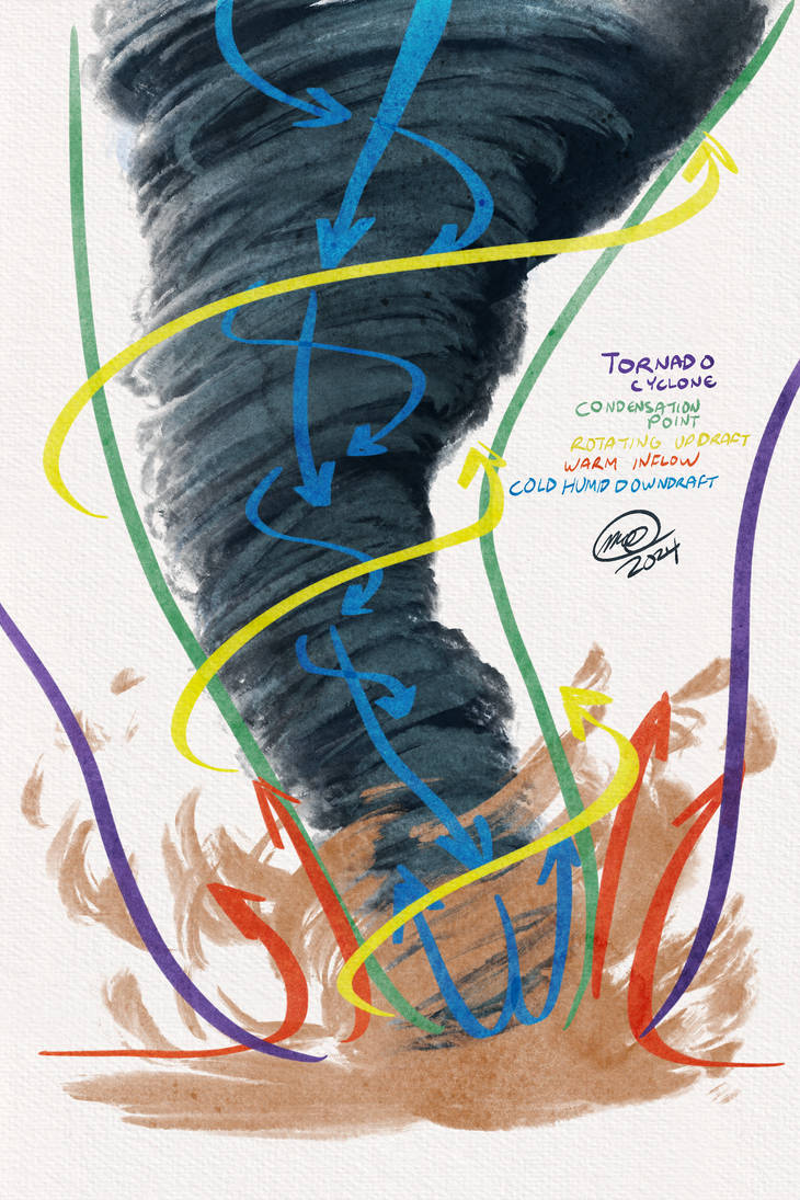
3 main tornado forces: orbit, up, and attraction.
Final Result:
My approach
My tornado consists of 5 node trees;
The Curve

This is the primary curve that acts as the foundation for the tornado, previewing the approximate movement and size of the tornado.
I begin by creating the main curve using the Curve node. Then, I resample it to generate points along the curve, allowing me to manipulate its shape and control the simulation. Afterward, I select the middle points, which will be the key focus for the movement dynamics.
To add some organic, shaky motion to the curve, I use the Attribute VOP node to generate simple noise. This noise serves as the perturbation that drives the curve’s movement. The setup inside the Attribute VOP node looks like this:

Tornado Part 1

This is where I begin setting up the node tree to generate the particles that will form the tornado. I start with a simple tube geometry, which I then blast and scatter into thousands of individual particles (Force Total Count: 50k).
Afterwards I create an attribute vop and call it noise.
Noise Attribute VOP
I choose my noise type to be sparse convolution noise and adjust it’s values to my liking.

Inside my attribute VOP I added a turbulent noise and exposed all of it’s parameters for easier access.

Attribute VOP ”Noise”
Forces that I needed to create for the tornado
- Up force (going upwards)
- Orbit Force (rotating around the middle)
- Attraction Force (keeping the particles in xyz distance to the centre to keep up the shape and form)
Combination of these 3 forces will create a vortex The Vortex Force DOP applies a vortex-like force on objects, causing them to orbit around a curve.

Vortex Particles DOP Network
After the Vortex Forces POP VOP node, I add a POP Wind node to simulate a real-life windy environment that influences the tornado, adjusting its swirl and amplitude attributes accordingly.
I also enable the use of VEXpressions. To create a more dynamic effect, I use the expression
amp *= @P.y / 50;, which multiplies the existing amplitude by the position along the Y-axis and divides by 50. This results in a more turbulent and realistic behavior for the tornado.

POP Wind Node
I follow up the POP Wind node with the Pop Kill Node to create a thin bounding box at the top of the tornado. This served to stop the particles from continuing to generate and allowed them to die out, preventing the tornado from forming indefinitely.

Pop Kill Bounding Box
Vortex Forces POP VOP

Inside my Vortex Forces POP VOP.
In my Vortex Forces POP VOP, I assign the curve path to a null node called “curve_points,” which I previously created in my curve geometry. This setup ensures that the node uses the curve as a reference, guiding the particles to spin around it.

Vortex Forces POP VOP Curve Path

Vortex Forces POP VOP Curve Path
Inside my Vortex Forces POP VOP (which essentially serves as a container for my forces, from which I can easily manipulate and adjust their values), I use the Point Cloud Open and Point Cloud Filter nodes to create the three main forces that shape my tornado: Attraction, Orbit, and Upward forces. I then connect each force to Ramp Parameter nodes, exposing their key parameters for easy manipulation. This allows me to easily adjust the tornado’s shape by tweaking the forces.
For instance, if I lower the attraction force, the tornado will become wider because the weaker attraction will pull it less towards the curve. Additionally, by adjusting the ramp so that the attraction force starts low, increases in the middle, and drops again at the top, the tornado will have a wider base and top with a narrower middle. This effect is achieved because the ramp points are connected to the curve points, influencing the shape accordingly. The goal of this was to create an easily manipulated preset for my tornado.
Point Cloud Open Node
The Point Cloud Open node in Houdini is used to access and read point cloud files, which typically contain 3D data represented as points with attributes. These files are often generated from 3D scanning processes or simulations where geometry is represented as a collection of points rather than a continuous mesh.
- Point Cloud Data: A point cloud is a set of points in 3D space, each with a position (x, y, z) and optional attributes like color, normal vectors, or other metadata.
- Opening a Point Cloud: The Point Cloud Open node imports and accesses this data, allowing you to work with it in Houdini. It supports common file formats such as
.pcd,.pts, or.bgeo.- Usage: Once the point cloud is loaded, you can process or analyze the points using various nodes. For example, you might sample attributes, calculate distances between points, or use the point cloud as a basis for generating more complex geometry.
In simple terms, the Point Cloud Open node allows Houdini to load point cloud data so you can use it in your project, such as importing a 3D scan for further manipulation or simulation.
Point Cloud Filter Node
The Point Cloud Filter node processes or modifies point cloud data, enabling you to refine or clean up the points for better results.
- Point Cloud Processing: This node works on point clouds that have already been imported into Houdini (e.g., via the Point Cloud Open node). It applies various filtering operations to improve the quality of the data.
- Types of Filtering:
- Noise Reduction: Removes outliers or irregular points that don’t fit the overall pattern, such as random noise from scanning or simulations.
- Smoothing: Adjusts the point distribution to make it more even or consistent.
- Decimation: Reduces the number of points in the cloud, simplifying the data while preserving the overall shape and details.
- Usage: After filtering, the cleaned-up point cloud can be used for further processing, such as generating a mesh, running simulations, or performing analysis.
In simple terms, the Point Cloud Filter node helps refine point cloud data by removing unwanted points or adjusting their positions, resulting in cleaner and more usable data.

Exposed parameters in my POP VOP: Forces

Exposed parameters in my POP VOP: Ramps

Exposed parameters in my POP VOP: Noise (Disabled in Tornado 1 as this one is just a smooth base, but will be used in Tornado 2 where I add the noise)
I return to my main (Tornado Part 1) network, and after the main DOP Network, I add an Attribute Delete node to remove any unnecessary attributes. The attributes I keep are the point attributes: velocity, color, age, and identifier.

Attribute Delete Node
Similarly, I then add a Group Delete node. Both actions are primarily performed for optimization, as they reduce the memory usage of the tornado simulation.

Group Delete Node
For further cleanup and optimization, I add a File Cache to store the simulation up to this point. This allows for instant and smooth playback later, instead of rendering frame by frame.

File Cache Node
Afterwards, I introduce the Timeshift node to skip the initial frames of the tornado forming, allowing me to start with the tornado already in its formation stage.

Timeshift Node
After the timeshift node, I decided finish to off this part of the graph with the null node called output particles

Following my particles output, I start working on my pyro and density sim. For that purpose, I add the pyro source node and add two main attributes: density & temperature.

Pyro Source Node
Followed by that, I add an attribute noise for my density attribute to further break up my shape.I choose my noise to be a perlin noise and adjust its values to my liking.

Attribute Noise Node
After that, I bring in the volume rasterize attributes node to actually view my smoke and attributes density and velocity. I Follow that up with a null node which creates an output for my density.

Volume Rasterize Attributes Node
After that I bring in a DOP Network and begin to work on final stage of my simulation

DOP Network Node
Inside my DOP Network, I bring in a pyro solver sparse node and connect a smoke object sparse to the first input, and volume source to the last.
In my Pyro Solver Sparse, I bring in my density and velocity fields

Velocity and Density field

Pyro Solver Sparse
The Tornado in the DOP network doesn’t have any light or shadows and is just a blank preview so outside of this geometry I bring in a skylight in order for the light to affect this. I use the DOP import node and choose any smoke object to view the tornado with lights and shadows like in a real environment.

DOP Import Tornado
Tornado Base
Tornado Part 2

In this section of the node tree, I create additional layers for the tornado, introducing more noise and turbulence to break up the flat, smooth appearance. The goal is to achieve a more organic and natural look, incorporating chaotic “mushrooming” effects that enhance the overall realism.
All three of these node trees are copied and pasted from my base tornado setup (Tornado Part 1, which I reviewed earlier). However, in these iterations, I utilize the noise attribute I created within the Vortex Forces POP VOP. When paired with other adjustments, this approach results in a significantly messier and more organic appearance.

Enabled Noise Setting which makes a big difference in the look of the tornado compared to the base version created earlier.
Tornado Bottom
I create the lower layer of dust and debris that’s commonly seen in tornadoes. This forms as the vortex picks up soil, grass, and other materials while spinning.
I start off with a grid as the base geometry followed by a mountain node to add some imperfections to the surface and animate the offset on it slightly.

Grid & Mountain Node
I then scatter it into particles and make the count 100000

Scatter Node
After the scattering process, I copy a significant portion of my initial graph (Tornado Part 1) and paste it into this section to save time. These nodes are highly adaptable and only require minor adjustments to fit seamlessly into this part of the workflow.

Result after copy pasting nodes from the first Tornado and adjusting certain areas.
Afterwards I turn my particles into vdb volumes

VDB converted into Volume
I follow that up with a DOP network for my simulation:

Tornado Particles
The tornado particles are modeled as thin, tube-like shapes that rotate around the tornado’s core. They simulate grass being carried along by the spinning vortex, mirroring how grass would move in a real tornado scenario.
━━━━━━━━━━━━━━━━━━━━━━━━━━━━━━━━━━━━━━
Week 1 – Introduction to Houdini
Keybinds:
-
Tab – look up things
-
Spacebar & G – zoom on view
-
G – Focus on the object
-
L – Tidy Up Graph
What is Houdini?
What is Houdini used for?
1. Complex Simulations
Houdini shines in simulating natural and dynamic phenomena. These simulations are a cornerstone of many VFX-heavy films. Some of the most common types of simulations in film include:
- Fire & Smoke (Pyro FX): Houdini’s pyro system is famous for its ability to create realistic fire, explosions, smoke, and other fluid dynamics. It’s used in films for scenes involving destruction, explosions, magical effects, or atmospheric elements like smoke or fog.
- Water and Fluids (FLIP Fluids): Houdini is used to simulate realistic water behavior, whether it’s flowing rivers, ocean waves, or the splash of water during an explosion or splashdown. It uses a specialized fluid solver called FLIP (Fluid-Implicit Particle) to create highly detailed and physically accurate simulations of liquids.
- Destruction (RBD/Soft Body Dynamics): When filmmakers need to show a building collapsing, an object breaking apart, or large-scale destruction (like a meteor hitting the ground), Houdini’s Rigid Body Dynamics (RBD) system helps simulate the shattering, breaking, and collapsing of objects in a realistic way. This is used in blockbuster action scenes (think of the crumbling buildings in Transformers or San Andreas).
- Cloth and Hair Simulations: For character clothing, capes, or hair, Houdini has robust tools for cloth and hair simulations. It’s used in films like The Jungle Book or Avengers: Endgame to create realistic movement of cloth, fabric, or hair that interacts with the environment and the character’s actions.
2. Particle Effects
Houdini’s particle system is extremely powerful for creating effects like dust, debris, rain, snow, and magical effects. In film, particles are often used to enhance the environment or to create surreal effects:
- Smoke, Explosions, and Dust: Particle effects can simulate the scattering of debris in an explosion, dust clouds from crumbling buildings, or even magical energy effects like force fields or mystical auras.
- Weather Effects: Particles are also used to create environmental effects, such as snowstorms, rain, lightning, and fog. These are all key to adding realism or atmosphere to scenes.
3. Crowd Simulations
For large-scale scenes involving crowds (think epic battle sequences like those in The Lord of the Rings or 300), Houdini’s crowd simulation tools allow animators to create vast numbers of characters without having to manually animate each one.
- Houdini can generate crowds that react to the environment, interact with each other, and follow a set of procedural rules. It’s incredibly useful for large battle scenes, stadium events, or even cityscapes where thousands of people are present.
4. Procedural Environments
Another major use of Houdini in film is the procedural generation of environments. It allows artists to build and manage vast, complex environments without manually constructing every individual element.
- For example, cityscapes, forests, or mountain ranges can be procedurally generated in Houdini using custom rules for placement, texture, and variation, resulting in lifelike environments that would take too long to build manually.
- Films like The Lord of the Rings trilogy and The Hobbit used procedural techniques for massive environments, like forests and mountain ranges, that had to be generated quickly and efficiently.
5. Creature Effects
Houdini is also used to create and simulate creatures, especially when those creatures need to interact with dynamic environments. This includes things like:
- Creature Animation: In films like Jurassic Park or Avatar, Houdini’s procedural tools help create lifelike animations for creatures, such as dinosaurs, dragons, or aliens, where the physical interaction with the environment (e.g., walking, running, swimming) needs to be dynamically simulated.
- Facial and Body Simulation: Houdini can simulate the deformation of skin and muscles, useful for creating realistic animation for characters, particularly for things like motion capture and facial expressions.
6. Environment Destruction
Large-scale destruction is another area where Houdini excels. Whether it’s buildings, vehicles, or entire landscapes, the software’s ability to handle and simulate destruction in a realistic, controllable way makes it invaluable for action-heavy films:
- Building Collapses: Movies like The Avengers series or The Day After Tomorrow feature scenes where entire buildings, cities, or landscapes collapse. Houdini’s destruction tools allow for the simulation of debris, fractures, and impacts in ways that make these scenes feel real and visceral.
- Natural Disasters: Houdini is also used for simulations of natural disasters, like earthquakes, tornadoes, or tsunamis. The software’s ability to handle massive, chaotic simulations is key to creating these jaw-dropping scenes.
7. Special Effects (Specialized FX)
Many films use Houdini to create specialized effects that don’t fall into traditional categories but are still essential for certain scenes:
- Magic Effects: For fantasy or sci-fi films, Houdini can be used to create magical effects like energy blasts, force fields, and other mystical phenomena. Films like Doctor Strange and Harry Potter make use of Houdini for these types of effects.
- Realistic Explosions and Collisions: Houdini’s detailed explosion simulations, including shockwaves, debris scattering, and fire, are used in action movies to create scenes that look both thrilling and realistic.
8. Compositing and Rendering Integration
While Houdini is best known for its procedural simulations and VFX, it also integrates well with other compositing and rendering software, making it part of the larger post-production pipeline. Houdini artists often work in tandem with compositors and lighting artists to integrate visual effects into final shots.
- Houdini can output data for use in Nuke (for compositing) or Maya (for character animation and modeling), and it works seamlessly with high-end render engines like Mantra, Arnold, and Redshift.
9. Virtual Production
With the rise of virtual production (used in films like The Mandalorian), Houdini plays a role in real-time effects and simulations. Unreal Engine, in particular, is used for creating real-time environments, and Houdini’s procedural systems can feed data directly into Unreal to dynamically generate environments, creatures, and other elements as the film is being shot.
10. High-Volume Asset Creation
Houdini is also used to automate the creation of large volumes of assets, whether it’s for background objects (like rocks, trees, or buildings) or even crowds of people. This is useful in large-scale visualizations, like battles, cities, or fantasy worlds that need to be populated with many assets without requiring individual manual work for every single one.
float – number that can be any number 2.3 -2 – infinity to infinity
vector is 3 floats XYZ
can represent velocity, colour (rgb)

Setting up the interface
In Houdini, the scale needs to be right and realsitic

Setting the realistic scale of the cheeseboard

Adding the UV unwrap node

Going into UV viewport

Adding the UV quickshade node so I can apply my texture onto the object

Relative reference

Importing another box onto my scene and adjusting the scale to that of a cheese block

Adding the colour node and setting it to yellow

Adding scatter node to scatter the cheese into many different points


━━━━━━━━━━━━━━━━━━━━━━━━━━━━━━━━━━━━━━
Week 2 – Domino
Excercise 1 – Domino Simulation
Final Result:

I create a geometry container called domino

I start off with a bezier curve and create the path for my domino

I resample my curve to create points which will indicate where the domino blocks will be


Copy the width of domino parameter and paste relative parameter in resample in lenght.
To view the tangent attribute, go into node info of ”resample node”.

Go into Visualisation > tangentu Point Attribute

tangent – direction
RBD Bullet Solver Node;
Collisions > Ground Plane so it doesn’t fall through the floor
━━━━━━━━━━━━━━━━━━━━━━━━━━━━━━━━━━━━━━
Week 3 – Fluid Simulations
Exercise 1
Final Result:
- I start off by creating 2 geometry nodes – one called emitter and one called collision geometry which will store my objects
- In emitter;
- I create a sphere for the emitter which is a polygon sphere followed up by a transform node to change some of its values
- In a separate DOP network, I setup flip solver, flip object and volume source.
- In my flip objects, I need to convert my spheres into particles

- In my source volume, I initialise source FLIP and select the SOP path to be my emitter output which will make the previously made sphere act as my source. I then play the animation but there’s no particles going out of it so I add gravity and that fixes it.
- The particles aren’t however colliding with my object so to fix that I bring in static object and static solver nodes
Emitter

I start off by creating two geometry nodes – one for the emitter and one for the collision geometry.

Inside the emitter geometry, I create a polygon sphere which will serve as my emitter core. I follow that up with a transform node to change some of its values and position.

I add a flipsource node to the sphere and make the voxel size 0.02 so that I can achieve good details.

I finish it off with a null node called Emitter_Output.
Collision Geometry

In my collision geometry, I add my capybara geometry which will serve as my collider. I follow it up with a transform node to make it a bit smaller and position it accordingly to my emitter.

I follow that up with a null node called Collision_Output.
Simulation


━━━━━━━━━━━━━━━━━━━━━━━━━━━━━━━━━━━━━━
Week 4 – Vellum Simulations
Things to consider when simulating cloth
- Substeps and Iterations
This will determine how stretchy the fabric is. For example 1 substep per 100 iterations will generally make the cloth very stretchy. A good starting point for clothing is 5 substeps, because that gives the solver a chance to work on a smaller timestep, which helps it resolve the energy in a more realistic fashion.
- Tailoring
Small alterations to the cloth could greatly improve the final look. For example, depending on the stride of your character, increasing the skirt width could prevent the garment from pulling at the bottom and give it a more interesting flow.
- Static
Often your garment can move around on the character in an unrealistic way, like it’s floating. Increasing the static coefficient will cause the garment to stick more to the character.
- Bend Strength
This parameter is what allows the individual triangles in the cloth to bend with respect to each other. A Bend Strength of 0 will result in lots of wrinkles, and a higher value will create a stiffer looking cloth.
- Compression Stiffness
This parameter allows the triangles to collapse, but not expand. This prevents small micro-wrinkles, because instead of having to fold over the cloth can just compress in place. A high value for compression will result in lot of crinkly detail.
- Tangent Stiffness
Turning on this parameter is useful when simulating pants or a skirt that’s attached to a character’s waist. Tangent stiffness holds the garment in place and prevents it from dropping or sliding down on the first frame due to gravity. It constrains the movement of the cloth in the direction tangent to the target geometry, and is better than decreasing the Rest Length Scale. It only works for Attach to Geometry constraints, which is Vellum geometry to external geometry, such as constraining cloth to a character’s body.
- Stiffness Dropoff
This parameter reduces or increases the stiffness of a constraint as it moves away from the rest state. It’s useful for creating glue constraints that lose stiffness as they’re stretched, or creating bend constraints that are weak to begin with and get stiffer as they bend away from their initial orientation. A Decreasing dropoff means that the stiffness starts at full strength and decreases to zero at the dropoff distance from the rest length. An Increasing dropoff means the stiffness starts at zero and increases to full stiffness at the specified distance from rest length.
- Air resistance
Air flow is very important to have with cloth. No air flow will cause the cloth to fall flat and too much air flow will cause the cloth to look like it’s being dragged. The default value of 0.1 usually produces good results.
- Gravity
Changing the gravity can make it appear as if time is going faster or slower. It can also affect scale, making things with lower gravity look bigger. Increasing gravity will also cause more stretching in the cloth, as stronger forces are pulling on it.
Exercise 1
Final Result:

I start off with a geometry node called ”Vellum Simulation” which will serve as a container for my geometry.

I add a 2×2 grid node with 50 rows and 50 collumns for good and detailed result.
- I then copy and transform the grid to make a few more pieces of cloth
- I add my test geometry which will be the collider for my cloth. I move it below the cloth pieces so that they can fall down on it.
- I add vellum cloth and vellum solver nodes to give it cloth behaviour.
- In vellum solver, I enable ground position and move it just below my test geometry.
- I use the connectivity node to split my objects into individual pieces 4 cloths and capybara geometry


━━━━━━━━━━━━━━━━━━━━━━━━━━━━━━━━━━━━━━
Week 5 – Plate & Noodles
Exercise 1 – Noodles
Final Result:

I create a geometry container called noodles.

Inside the geometry container, I pull out the sphere node and set it to polygons.

I follow that up by a transform node to move it a bit up.

Then, I add a popnet DOP network to turn everything into particles.

Inside of the DOP network.

I add gravity after the popsolver node to make the particles fall.

Followed by the gravity node, I add a ground plane and merge it into my main graph so that the particles stop falling as they hit the ground.
In my POP source, I set the emission type to all points so that the particles only emit from the spheres points.

I go back to my parent network and in my transform node I animate rotation of my source fo rmore interesting and varied simulation

I add a pop drag node to add some air resistance

I add an attribute wrangle to further manipulate my particles with the code of @v = @P which means that the velocity will equal position and convert point number into point id

In my pop grains node, I disable use open gl in solver and
In my POP Source Birth tab, i set a keyframe on a frame where I want the particles to stop generating and go a keyframe after that and set the impulse activation to 0
Plate Graph
- curve
- resample: 0.001
- revolve: ensure unique seam vertices / divisions:100
- fuse: no changes / function of the node – merge in the middle
- remesh: target size: 0.002
- uv project: initialize
- uv quick shade – choose texture

UV quick shade: I apply the texture onto my object.
null
stage > sop import > sop path > null:plate
karma xpu render
━━━━━━━━━━━━━━━━━━━━━━━━━━━━━━━━━━━━━━
Week 6 –
━━━━━━━━━━━━━━━━━━━━━━━━━━━━━━━━━━━━━━
Week 7 – Destruction
Exercise 1
Final Result:

I start off with a simple 3×3 sized grid.

I then resample it to create points on my geometry so that I can further manipulate it.
Floors

RBD Material Fracture
I set my material type as concrete and enable chipping to create little chip pieces
RBD Bullet Solver
Collision – ground collision – turn on ground plane
Constraints
constrain strength is the little knits that pull the geometry together. if it is too strong the geometry won’t fall aport hence why u need to make it lower and same applies for chipping glue strength.
The chips first start to fall out of the building until the entire building starts going down.
Explosion
I select my bottom points so that only those can be affected by the explosion then I add point velocity and enable conical noise for a good explosion simulation.
File Cache
At the very end of my project, I cache it so that I won’t have to deal with long render times every time I want to replay the animation.


Exercise 2


Packed Geometry won’t collide with things properly, hence we have to unpack it
━━━━━━━━━━━━━━━━━━━━━━━━━━━━━━━━━━━━━━
Week 9 – Destruction
Geo -> Null -> Edit Parameter Interface [add unit width, unit depth, storey height, column width, floor thickness, wall thickness – float, number of storeys – interger]

